This challenge is a standard supervised learning problem. The dataset includes application data for every loan given over a 6 month period.
There are 4 tabs with data, labeled "trainX", "trainY", "testX" and "testY". The train tabs contain the first 4.5 months of loans, while the test tabs have loan data from the following 1.5 months.
trainY and testY contain the targets. They represent whether the loans were fully funded (TRUE values) or partially funded (FALSE values). The fully funded values are withheld from testY, and your job will be to fill them in.
Use trainX and trainY to build a model to predict whether or not future loans will be fully funded. You should then use your model on the data from testX to make new predictions. We’ll score those predictions against the true values of testY to see how well your model performs.
This is intended to be a fairly straightforward task. I didn’t intentionally include any big surprises or “gotchas”. I hope that your model performs well, but it’s even more important that your approach is sound and you avoid major mistakes.
Please put your predictions in column B of the "testY" tab. The predictions should be made such that higher values are more likely to be TRUE and lower values more likely FALSE.
Pleae include a short description of which evaluation metric you selected & why.
Data Dictionary
| Variable | Definition | Type |
|---|---|---|
| customer_id | unique customer id | alphanumeric |
| status | was customer approved or denied | String |
| residence_rent_or_own | customer is renting | Boolean |
| monthly_rent_amount | monthly rent amount | Numeric |
| bank_account_direct_deposit | customer signed up for direct deposit | Boolean |
| application_when | date when customer applied for a loan | MM/DD/YY HH:MM |
| loan_duration | term of loan | Numeric |
| payment_ach | has customer signed up for ACH payments | Boolean |
| num_payments | # of payments made by customer | Numeric |
| address_zip | customer resident zip code | Numeric |
| bank_routing_number | customer bank routing number | Numeric |
| home_phone_type | type of customer phone | String |
| monthly_income_amount | customer monthly income amount | Numeric |
| raw_l2c_score | Third party score | Numeric |
| raw_FICO_telecom | Third party score | Numeric |
| raw_FICO_retail | Third party score | Numeric |
| raw_FICO_bank_card | Third party score | Numeric |
| raw_FICO_money | Third party score | Numeric |
| FullyFunded | Fund customer | Boolean |
Good luck!
import pandas as pd
import numpy as np
import seaborn as sns
import matplotlib.pyplot as plt


import random
from sklearn.metrics import roc_curve, auc
from sklearn.model_selection import cross_val_score
from sklearn.model_selection import KFold
from sklearn.model_selection import GridSearchCV


# Importing the various models

from sklearn.tree import DecisionTreeClassifier
from sklearn.ensemble import RandomForestClassifier
from sklearn.linear_model import LogisticRegression
from sklearn.linear_model import Lasso, Ridge
from sklearn.neighbors import KNeighborsClassifier
from sklearn.ensemble import GradientBoostingClassifier
import xgboost as xgb
from sklearn.svm import SVC

# Ensemble model
from sklearn.ensemble import VotingClassifier


# Import sklearn
from sklearn import feature_selection, linear_model
import warnings
warnings.filterwarnings('ignore')

%matplotlib inline
Loading train and test data.
sheets = ['trainX','trainY','testX','testY']

trainX = pd.read_excel("HW3Data.xlsx", sheetname='trainX')
trainY = pd.read_excel("HW3Data.xlsx", sheetname='trainY')
testX = pd.read_excel("HW3Data.xlsx", sheetname='testX')
testY = pd.read_excel("HW3Data.xlsx", sheetname='testY')

trainX.head()
trainY.head()
trainX.shape
print("Dataset shape: {}, {}".format(trainX.shape[0], trainX.shape[1]))
# Info about data set, datatype
trainX.info()
# Checking for missing values
trainX.isnull().sum()
Turns out to be no missing values, so no need to impute data.
# Check customer id is same for features & target
print("Is customer ID same for feature & target? (training)", (pd.Series.equals(trainX.customer_id, trainY.customer_id)))
print("Is customer ID same for feature & target? (test)", (pd.Series.equals(testX.customer_id, testY.customer_id)))

# Check if columns are the same/same order
trainX.columns == testX.columns
# Checking for any quirks
trainX.describe()
# Number of categorical columns
print("Number of categorical columns:", len(trainX.describe(include=['object']).columns))
trainX.describe(include=['object', 'datetime64'])
# Plotting univariate distributions to check for skew, patterns, types of distribution
trainX.hist(layout = (3,6), figsize = (14,9), bins = 20);

Some graphs show a right skew (monthly_income_amount, monthly_rent_amount, num_payments). Others are categorical such as if someone rents or owns, or loan duration.
sns.pairplot(trainX)
plt.show()

trainX.plot(kind='density', subplots=True, layout=(3,6), figsize=(14,9), sharex=False);

# Looking for skew
trainX.skew()
# Checking when these applications were submitted, find the time range
trainX.application_when.sort_values()
# Checking longest loan duration, appears to be 8 [years?] -- most common is 5 year loan
# trainX.loan_duration.sort_values(ascending=False)
trainX.loan_duration.value_counts()
Idea: Is it possible to add years (loan duration) to the date loan was applied for? Maybe to see if you can weigh number of payments strongly.
# Checking address_zip, see if there is an imbalance in where these people live
trainX['address_zip'].value_counts()
Shows 146 different address_zip values.
# Checking string and other variables.
print(trainX.status.value_counts())
print("******************")
trainX.bank_account_direct_deposit.value_counts()
Noticed that all loans in trainX are approved. I checked with testX and it is also the same. There are more than 4 times the amount of people who use direct deposit than not.
corr = trainX.corr()
# plot correlation matrix
corr = trainX.corr()
sns.heatmap(corr,
           xticklabels=corr.columns.values,
           yticklabels=corr.columns.values);

There are a lot of highly correlated variables, particularly when it comes to the credit scores.
So maybe need to drop some of them?
A possible approach would be to check their coefficients and p-values, and pick a FICO score.
Note: Averaging would probably remove the differences, so I will not be doing that. (From Aug. 27 office hours)
Checking for "best" FICO score using the get_linear_model_metrics from the linear regression notebook.
def get_linear_model_metrics(X, y, algo):
    # Get the pvalue of X given y. Ignore f-stat for now.
    pvals = feature_selection.f_regression(X, y)[1]
    # Start with an empty linear regression object
    # .fit() runs the linear regression function on X and y
    algo.fit(X,y)
    residuals = (y-algo.predict(X)).values

    # Print the necessary values
    print('P Values:', pvals)
    print('Coefficients:', algo.coef_)
    print('y-intercept:', algo.intercept_)
    print('R-Squared:', algo.score(X,y))

    # Plot residuals
#     h = sns.residplot(X,y)
#     h.set(xlabel="ah")

    # Keep the model
    return algo

# lm = get_linear_model_metrics(X, y, lm)


# The set of variables I will be checking coefficient, p-value, r-squared values:
x_sets = (
    ['raw_l2c_score'],
    ['raw_FICO_telecom'],
    ['raw_FICO_retail'],
    ['raw_FICO_bank_card'],
    ['raw_FICO_money'],
    ['raw_l2c_score', 'raw_FICO_telecom'],
    ['raw_l2c_score', 'raw_FICO_retail'],
    ['raw_l2c_score', 'raw_FICO_bank_card'],
    ['raw_l2c_score', 'raw_FICO_money'],
    ['raw_FICO_money','raw_FICO_bank_card']
)

# Using logistic regression as the linear model
for x in x_sets:
    print(', '.join(x))
    get_linear_model_metrics(trainX[x], trainY.FullyFunded, linear_model.LogisticRegression())
    print()
I opted to use raw_FICO_telecom since it accounts for utility and phone bills, and it returned the highest R-Squared value (albeit barely squeezed out the highest at 0.7325 compared to 0.73). Also it appears to show that adding more than one credit score does not contribute changes to the R-Squared value. Seems useful for people new to credit.
I will try to do a raw_l2c_score to raw_FICO_telecom ratio or something like that. From searching online, the l2c score appears to be a way to score people with little to no credit history.
Source: http://money.cnn.com/2015/04/02/pf/new-fico-credit-score/index.html
Removing columns that may not have anything to do with whether a loan is fully funded.
Removing home_phone_type, bank routing number, customer id, status
# Home phone type
trainX.home_phone_type.value_counts()
# Bank routing number
# customer_id
# status - all loans are Approved in this dataset and the testX dataset.
Going to use credit scores as primary predictors of whether or not they will be fully funded.
Checking for quirks in their distributions.
f, axarr = plt.subplots(3, 2, figsize=(14, 10));
# funded = trainY.FullyFunded.values

axarr[0,0].hist(trainX['raw_l2c_score'].values, bins = 20)
axarr[0,0].set_title('raw_l2c_score');

axarr[0,1].hist(trainX['num_payments'].values, bins = 20)
axarr[0,1].set_title('raw_FICO_telecom');

axarr[1,0].hist(trainX['raw_FICO_retail'].values, bins = 20)
axarr[1,0].set_title('raw_FICO_retail');

axarr[1,1].hist(trainX['raw_FICO_bank_card'].values, bins = 20)
axarr[1,1].set_title('raw_FICO_bank_card');

axarr[2,0].hist(trainX['raw_FICO_money'].values, bins = 20)
axarr[2,0].set_title('raw_FICO_money');

axarr[2,1].hist(trainX['monthly_income_amount'].values, bins = 20)
axarr[2,1].set_title('monthly_income_amount');

f, axarr = plt.subplots(3, 2, figsize=(10, 9))
funded = trainY.FullyFunded.values
axarr[0, 0].scatter(trainX.num_payments.values, funded)
axarr[0, 0].set_title('num_payments');
axarr[0, 1].scatter(trainX.raw_FICO_telecom.values, funded)
axarr[0, 1].set_title('raw_FICO_telecom');
axarr[1, 0].scatter(trainX.monthly_rent_amount.values, funded)
axarr[1, 0].set_title('monthly_rent_amount');
axarr[1, 1].scatter(trainX['raw_l2c_score'].values, funded)
axarr[1, 1].set_title('raw_l2c_score');
axarr[2, 0].scatter(trainX.raw_FICO_bank_card.values, funded)
axarr[2, 0].set_title('raw_FICO_bank_card');
axarr[2, 1].scatter(trainX.raw_FICO_retail.values, funded)
axarr[2, 1].set_title('raw_FICO_retail');

Perhaps people who consistently make payments (num_payments) are more likely to get funding? Could be a contributor to credit history. Wanted to see if there was anything with that, but nothing noticeable showed up in these plots.
What about categorizing into levels of FICO score? Using get dummies to assign 0 & 1 to the various levels.
Figuring out how to assign scores by credit level.
Creating tiers based off the original FICO Score
- Exceptional, Very Good, Good, Fair, Very Poor
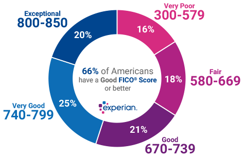
Assigning 4 levels of mean credit score:
- Exceptional (800-850)
- Very Good (740 to 799)
- Good (670 to 739)
- Fair (580 to 669)
- Very Poor (579 and below)
train_X = trainX.copy() # train_X is the copy dataset!

def fico_telecom_level(df):
    df.loc[df['raw_FICO_telecom'].between(800,850), 'credit_level'] = 'exceptional'
    df.loc[df['raw_FICO_telecom'].between(740,799), 'credit_level'] = 'very good'
    df.loc[df['raw_FICO_telecom'].between(670,739), 'credit_level'] = 'good'
    df.loc[df['raw_FICO_telecom'].between(580,669), 'credit_level'] = 'fair'
    df.loc[df['raw_FICO_telecom'].between(0,579), 'credit_level'] = 'very poor'

    return df

def credit_dummies(df):
    credit_level_dummies = pd.get_dummies(df['credit_level'], prefix='credit')
    df = pd.concat([df, credit_level_dummies], axis=1)
    df.drop('credit_level', axis=1, inplace=True)

    return df

# Dropping features that don't seem to be very predictable
def drop_features(df):
    dropCols = ['bank_routing_number', 'customer_id', 'home_phone_type','status','address_zip',
               'application_when','bank_account_direct_deposit', 'payment_ach',
               'residence_rent_or_own']

    df = df.drop(dropCols, axis = 1, inplace = True)
    return df

# Dropping the credit score columns
def drop_credit(df):
    creditCols = ['raw_l2c_score','raw_FICO_retail', 'raw_FICO_bank_card','raw_FICO_money'] # no raw_FICO_telecom
    df = df.drop(creditCols, axis = 1, inplace = True)
    return df

# Checking to see if training data set copy is same as original
train_X.head()
# Applying functions to training data set.
drop_features(train_X)
drop_credit(train_X)
train_X = credit_dummies(fico_telecom_level(train_X)) # needs to be assigned to save the dataframe result.

# Check to see if functions transformed dataset successfully.
train_X.head()
Was not able to apply get_dummies inside a function for some reason.
Going to apply it separately.
Trying out CART as my first model.
scoring = 'roc_auc'
num_folds = 5
seed = 10
kfold = KFold(n_splits = num_folds, random_state = seed)
y = trainY['FullyFunded'] # Extract target (FullyFunded), not customer_id.

model = DecisionTreeClassifier(random_state = seed)
# Fits the model
model.fit(train_X, y)

scores = cross_val_score(model, train_X, y, cv = kfold, scoring = scoring)
print('CV AUC {}, Avg. AUC {}'.format(scores, scores.mean()))
Tweaking CART model parameters. Picked these two values for max_depth & min_samples leaf based off the class we looked over the StumbleUpon data.
model = DecisionTreeClassifier(
                max_depth = 4,
                min_samples_leaf = 5, random_state = seed)

model.fit(train_X, y)
scores = cross_val_score(model, train_X, y, cv = kfold, scoring = scoring)
print('CV AUC {}, Avg. AUC {}'.format(scores, scores.mean()))
Changing the max_depth and min_samples_leaf results in a 10% increase in AUC score.
features = train_X.columns
feature_importances = model.feature_importances_

features_df = pd.DataFrame({'Features': features, 'Importance Score': feature_importances})
features_df.sort_values('Importance Score', inplace=True, ascending=False)

features_df.head(20)
Turns out the indicator columns I created turned out to be nonfactors in the model.
Although the FICO telecom score is based off the original FICO score with the same score range, it
did not contribute anything meaningful to the model.
Evaluating various models' performances
def model_performance(df):
    scoring = 'roc_auc'
    num_folds = 5
    seed = 10
    kfold = KFold(n_splits = num_folds, random_state = seed)

    results = []
    names = []
    models = []

    # Tweak CART ---- max_depth = 4, min_samples_leaf = 5,
    models.append( ('CART', DecisionTreeClassifier(random_state = seed)) )
    models.append( ('CART v2', DecisionTreeClassifier(random_state = seed, max_depth = 4, min_samples_leaf = 5)) )
    models.append( ('RandomForestClassifier', RandomForestClassifier(random_state = seed)) )
    models.append( ('LogisticRegression', LogisticRegression(random_state = seed)) )
    models.append( ('SVC', SVC(random_state = seed)) )
    models.append( ('GradientBoostingClassifier', GradientBoostingClassifier(random_state = seed)) )
    models.append( ('KNeighborsClassifier', KNeighborsClassifier()) )
    models.append( ('XGBClassifier', xgb.XGBClassifier(seed = seed)) )


    for name, model in models:
        kfold = KFold(n_splits = num_folds, random_state = seed)

        names.append(name)
        model.fit(df, trainY['FullyFunded'])

        scores = cross_val_score(model, df, trainY['FullyFunded'], cv = kfold, scoring = scoring)
        results.append(scores)

        msg = "{}: {} ({})".format(name, scores.mean(), scores.std())
        print(msg)
        print()
    return df
model_performance(train_X)
scoring = 'roc_auc'
num_folds = 5
seed = 10
kfold = KFold(n_splits = num_folds, random_state = seed)


results = []
names = []
models = []

# CART v2 is the modified CART ---- max_depth = 4, min_samples_leaf = 5,
models.append( ('CART', DecisionTreeClassifier(random_state = seed)) )
models.append( ('CART v2', DecisionTreeClassifier(random_state = seed, max_depth = 4, min_samples_leaf = 5)) )
models.append( ('RandomForestClassifier', RandomForestClassifier(random_state = seed)) )
models.append( ('LogisticRegression', LogisticRegression(random_state = seed)) )
models.append( ('SVC', SVC(random_state = seed)) )
models.append( ('GradientBoostingClassifier', GradientBoostingClassifier(random_state = seed)) )
models.append( ('KNeighborsClassifier', KNeighborsClassifier()) )
models.append( ('XGBClassifier', xgb.XGBClassifier(seed = seed)) )


for name, model in models:
    kfold = KFold(n_splits = num_folds, random_state = seed)

    names.append(name)
    model.fit(train_X, trainY['FullyFunded'])

    scores = cross_val_score(model, train_X, trainY['FullyFunded'], cv = kfold, scoring = scoring)
    results.append(scores)

    msg = "{}: {} ({})".format(name, scores.mean(), scores.std())
    print(msg)
    print()
Refinement Workflow Results - Trial 1
| Model Description | Local CV (Std Dev) |
|---|---|
| Baseline: CART | 0.6176 (0.0558) |
| CART v2: Modified parameters | 0.7172 (0.1002) |
| RandomForestClassifier | 0.7136 (0.0620) |
| Logistic Regression | 0.7001 (0.0506) |
| SVC | 0.5073 (0.0247) |
| GradientBoostingClassifier | 0.7122 (0.1067) |
| KNeighborsClassifier | 0.5684 (0.0541) |
| XGBClassifier | 0.7412 (0.0745) |
It appears to be that with a training dataset of only 7 columns, XGBClassifier scores the highest.
The engineered features in this first test were one hot encoded credit score tiers (exceptional, very good, good, fair, very poor), and did not end up contributing to the CART model.
Feature Engineering (FE)
- Created a payment_loan_ratio that divides number of payments by loan duration. Perhaps making more payments is indicative of getting a fully funded loan. In a previous scatterplot above, num_payments did not show any correlation with becoming FullyFunded. Although making more payments over the course of a loan could build credit.
- Created an income_rent_difference feature, which shows how much income a person has left over after subtracting their rent payment for the month. People who have more leftover money could be more likely to make their loan payments.
- Created a raw_FICO_telecom to raw_l2c_score ratio since both scores appear to be measures of people who are new to having credit (meaning they have little to no credit history). Settled on using that since raw_l2c_score had a higher max value in the dataset.
- Used describe() on raw_l2c_score & raw_FICO_telecom to check.
# Feature Engineering (FE)
def first_order_FE(df):
    df["payment_loan_ratio"] = df.apply(payment_loan_ratio, axis=1)
    df["income_rent_difference"] = df.apply(income_rent_difference, axis=1)
    df["telecom_l2c_ratio"] = df.apply(telecom_l2c_ratio, axis=1)
    return df

def payment_loan_ratio(df):
    return df.num_payments / df.loan_duration

def income_rent_difference(df):
    return df.monthly_income_amount - df.monthly_rent_amount

def telecom_l2c_ratio(df):
    return df.raw_FICO_telecom / df.raw_l2c_score
One additional method to feature engineer is to predict negative income, see how their monthly income changes from month to month. Data is not available though.
- A shortcoming of income_rent_difference is that we do not know the person's housing situation.
- If they split rent, then it possible to have a higher rent than income.
- Also the residence_rent_or_own variable is very strange.
Transforming the dataset using feature engineering.
# Dropping different credit score columns
def drop_credit_FE(df):
    creditCols = ['raw_FICO_retail', 'raw_FICO_bank_card','raw_FICO_money'] # no raw_FICO_telecom or raw_l2c_score
    df = df.drop(creditCols, axis = 1, inplace = True)
    return df
train_X2 = trainX.copy()
first_order_FE(train_X2)
drop_features(train_X2)
drop_credit_FE(train_X2)
print("Data shape is:",train_X2.shape)
train_X2.head()
Evaluating Model Performances (Test 2)
model_performance(train_X2)
| Model Description | Performance 2 - Performance 1 | Change in CV Score |
|---|---|---|
| Baseline: CART | 0.6394 - 0.6176 | 0.0218 |
| CART v2: Modified parameters | 0.7199427737 - 0.7172 | 0.0027 |
| RandomForestClassifier | 0.7034117022 - 0.7136 | -0.01018 |
| Logistic Regression | 0.6996489925 - 0.7001 | -0.0004510 |
| SVC | 0.503425254 - 0.5073 | -0.003874 |
| GradientBoostingClassifier | 0.7310378055 - 0.7122 | 0.01883 |
| KNeighborsClassifier | 0.522819633 - 0.5684 | -0.04558 |
| XGBClassifier | 0.749506304 - 0.7412 | 0.008306 |
Overall, only very slight changes in model performances. The baseline model increased by 2%, GradientBoostingClassifier performance improved by 1.88 % while the modified CART (CART v2), and XGBClassifier increased less than a hundredth.
Next is model tuning!
Decided on tuning GradientBoostingClassifier & XGBClassifier!
Local CV performance function
def local_cv(model, params, printFeatureImportance=True):
    param_grid = params
    kfold = KFold(n_splits = num_folds, random_state = seed)
    grid = GridSearchCV(estimator=model, param_grid=param_grid, scoring=scoring, cv=kfold)
    grid_result = grid.fit(train_X2, trainY.FullyFunded)

    # Plotting the Feature Importances
    if printFeatureImportance:
        predictors = [x for x in train_X2.columns] # Every x column
        feat_imp = pd.Series(grid_result.best_estimator_.feature_importances_, predictors).sort_values(ascending=False)
        feat_imp.plot(kind='bar', title='Feature Importances')
        plt.ylabel('Feature Importance Score')
        # Dataframe of features
        features_df = pd.DataFrame({'Features': predictors, 'Importance Score': grid_result.best_estimator_.feature_importances_})
        features_df.sort_values('Importance Score', inplace=True, ascending=False)

    print("Best: %f using %s" % (grid_result.best_score_, grid_result.best_params_))
    print()
    for params, mean_score, scores in grid_result.grid_scores_:
        print("%f (%f) with: %r" % (scores.mean(), scores.std(), params))

    return features_df
GradientBoostingClassifier
GradientBoostingClassifier().get_params().keys()
Using default parameters for GradientBoostingClassifier.
params = {"learning_rate": [0.1],
          "n_estimators": [100],
          "min_samples_split": [2],
          "min_samples_leaf": [1],
          "max_depth": [3]}
local_cv(GradientBoostingClassifier(random_state = seed), params)

Using tuned parameters for GradientBoostingClassifier.
params = {"max_depth": [5],
          "n_estimators": [150],
          "min_samples_split": [2],
          "min_samples_leaf": [7],
          "learning_rate": np.arange(0.01, 0.101, 0.01),}

local_cv(GradientBoostingClassifier(random_state = seed), params)

Able to make a 3% improvement in score by tuning parameters.
When examining the two feature importances plots, the importance of payment_loan_ratio increases in the tuned model; however, it also brings up the scores of the other features as well so it doesn't rely as much on one feature.
Tweaking the learning rate.
Found that 0.0409999 --> rounded to 0.041 gives us the best score.
params = {"max_depth": [5],
          "n_estimators": [150],
          "min_samples_split": [2],
          "min_samples_leaf": [7],
          "learning_rate": [0.041],
          "max_features": ['auto']}


local_cv(GradientBoostingClassifier(random_state = seed), params)

Tweaking the learning rate gets us even more of an even distribution of importance scores among the features.
xgb.XGBClassifier().get_params().keys()
params = {"max_depth": [3],
          "n_estimators": [100],
          "min_child_weight": [7]}

local_cv(xgb.XGBClassifier(seed = seed), params)

Creating ensemble model and submitting prediction
First, the test dataset needs to be transformed. Using the feature engineering functions created to transform the dataset.
first_order_FE(testX)
drop_features(testX)
drop_credit_FE(testX)
print("Data shape is:", testX.shape)
testX.head()
# Create the sub models. Using XGBClassifier & GradientBoostingClassifier
estimators = []

model1 = xgb.XGBClassifier(n_estimators = 100, min_child_weight = 7, max_depth = 3)
estimators.append(('XGBClassifier', model1))

model2 = GradientBoostingClassifier(max_depth = 5, n_estimators = 150,
                                    min_samples_split = 2,
                                    min_samples_leaf = 7,
                                    learning_rate = 0.041,
                                    max_features = 'auto')
estimators.append(('GradientBoostingClassifier', model2))


# Creating ensemble model
ensemble = VotingClassifier(estimators, voting='soft')
results = cross_val_score(ensemble, train_X2, trainY.FullyFunded, cv = kfold)

# Printing results
print("CV Scores: {} // Mean Score: {} // Std Dev: {}".format(results, results.mean(), results.std()))
print()

# Fitting model then making a prediction
ensemble_result = ensemble.fit(train_X2, trainY.FullyFunded)
ensemble_preds = ensemble_result.predict(testX)

print("Estimators variable:\n", estimators)
print()
print(ensemble)
Submission to CSV file
submission = pd.DataFrame({"customerId": testY.customer_id, "FullyFunded": ensemble_preds})
submission.to_csv("HW3_Final_Predictions.csv", index = False)
Final Workflow Results
Workflow Results - Trial 1: One Hot Encoded Credit Score Levels
| Model Description | Local CV (Std Dev) |
|---|---|
| Baseline: CART | 0.6176 (0.0558) |
| CART v2: Modified parameters | 0.7172 (0.1002) |
| RandomForestClassifier | 0.7136 (0.0620) |
| Logistic Regression | 0.7001 (0.0506) |
| SVC | 0.5073 (0.0247) |
| GradientBoostingClassifier | 0.7122 (0.1067) |
| KNeighborsClassifier | 0.5684 (0.0541) |
| XGBClassifier | 0.7412 (0.0745) |
It appears to be that with a training dataset of only 7 columns, XGBClassifier scores the highest.
The engineered features in this first test were one hot encoded credit score tiers (exceptional, very good, good, fair, very poor), and did not end up contributing to the CART model when looking at feature importances.
Workflow Results - Trial 2: With Feature Engineering
| Model Description | Performance 2 - Performance 1 | Change in CV Score |
|---|---|---|
| Baseline: CART | 0.6394 - 0.6176 | 0.0218 |
| CART v2: Modified parameters | 0.7199427737 - 0.7172 | 0.0027 |
| RandomForestClassifier | 0.7034117022 - 0.7136 | -0.01018 |
| Logistic Regression | 0.6996489925 - 0.7001 | -0.0004510 |
| SVC | 0.503425254 - 0.5073 | -0.003874 |
| GradientBoostingClassifier | 0.7310378055 - 0.7122 | 0.01883 |
| KNeighborsClassifier | 0.522819633 - 0.5684 | -0.04558 |
| XGBClassifier | 0.749506304 - 0.7412 | 0.008306 |
Workflow Results - Trial 3: Using GridSearch and Ensemble (w/ Feature Engineering)
| Model Description | Local CV (Std Dev) |
|---|---|
| GradientBoostingClassifier (Default Parameters) + feature engineering | 0.731038 (0.073714) |
| GradientBoostingClassifier + feature engineering & tuning | 0.776827 (0.084874) |
| GradientBoostingClassifier + feature engineering & additional learning rate tuning | 0.779260 (0.07950) |
| XGBClassifier + feature engineering & tuning | 0.769292 (0.037175) |
| Ensemble XGBClassifier and GradientBoostingClassifier (feature engineering and tuning) | 0.8025 (0.03259601202601321) |